Best route to the vet’s office
Our cat Bagheera doesn’t actually mind going to the vet’s office that much. But the drive to the vet’s office is another story; Baggy squawks the whole ride there, whether he’s in a cat carrier or on a leash in the car. Thankfully, it’s less than a mile from our house to the vet. This leads to the question “What’s the fastest way to get from our house to the vet?”
Of course, this is really just a toy problem. The “best” route to the vet is probably a slower one with a smoother drive, rather than the fastest drive (the fastest drive surely involves hoonin’ a motorcycle, which definitely does not lend itself to calming the cat). I don’t expect there to be a substantial difference between the routes under consideration anyway. Nevertheless, should be a fun little problem to play with for a little bit.
I’ve put together a little notebook to mess around with this problem. You can download the notebook and run it for yourself, in which case you’ll need the neighborhood graph file. Alternatively, you can view the code and output as a static webpage.
The neighborhood is set up in a near perfect grid. However, it’s a total hodge podge of two-way stop signs, so the fastest path is more complicated, and I expect the dominant factor to be the number of stop signs encountered along the route. Looking on OpenStreetMap (OSM), there are some stop signs that are labeled, but many are missing and some are not quite correct. I’ve been thinking of contributing to OSM, since I use it so often for routing for dirt biking, so I finally created an account. They’ve got a pretty slick online editor (iD) that makes it quick and easy to fix up the signage. I spent a couple hours going taking a quick tutorial on the editor, figuring out how they’d like stop signs entered, and entering in all the stop signs.
Geoff Boeing has developed a super handy Python package OSMNx for working with OSM data with NetworkX. I used it to pull the OSM street data in a box surrounding our ‘hood. OSMNx does a good job of removing non-intersection nodes while preserving the shape of “ways” (in OSM jargon).
bbox_north = ...
bbox_south = ...
bbox_east = ...
bbox_west = ...
G_simple = osmnx.graph_from_bbox(bbox_north, bbox_south, bbox_east, bbox_west,
                                 network_type='drive_service', simplify=True)
osmnx.plot_graph(G_simple, node_size=20);
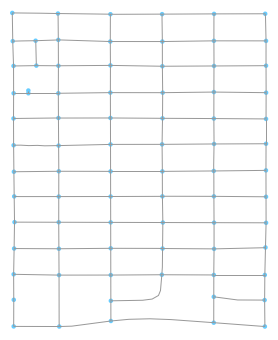
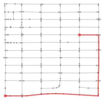
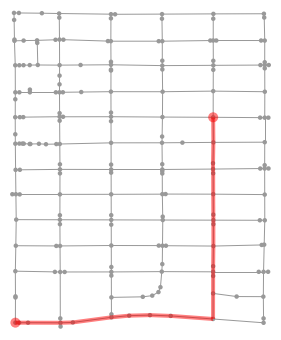
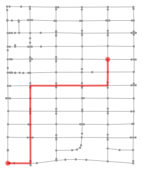
Due to the location of the vet’s office, all good paths to the vet will go through the lowest, leftmost node in the graph above. The rest of the route goes just a bit further South and ends at the vet. So all routes will start at home and head Southwest.
First hack at it
OSM provides (and OSMNx pulls) some extra data for each node and edge/way in the graph.
These extra data include lat/lon, length of the way, and presence (and direction) of stop signs.
Let’s say we average 20 mph on residential roads, 10 mph on alleyways/service roads, and it takes 5 seconds per stop sign encountered.
We can then estimate the time it takes to traverse each edge, plus 5 seconds for each node with a stop sign, and use that to weight each edge of the graph.
We now have a weighted undirected graph, so we can use Dijkstra (as implemented in nx.shortest_path) to find the shortest path from home to the vet.

Note a couple things:
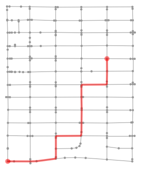
- In the above figure, I’m using the unsimplified graph. This is done so that we get all the two-way stops, which are shown as pairs of nodes slightly above & below, or left & right of the intersection node.
- The two-way stops are potentially double counted, since I’m adding 5 seconds each time we hit a node with a stop sign. But at two-way stops, one sign is forward facing and the other is backward facing, so doesn’t affect our movement.
Slight improvement
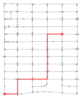
In OSM, each edge/way is actually directional, which enables stop signs at two-way intersections to have a directionality. We can use this to do a better job of handling the stop signs (i.e., not double counting them). Below are the top 6 fastest times and paths, arranged from left to right in reading order. Interestingly, the best path with the improved metric is same as with the earlier metric.
The top three routes have nearly equal times.
If we treat the streets as forming a perfect grid, the top three paths should have identical times.
The difference comes from the length tag provided by OSM; indeed, the top three paths each have three stop signs (not counting the source and target nodes) but slight differences in total length.
The next three paths are almost four seconds longer, which comes from an additional stop sign (five seconds) and a shorter path.
| 115.73 | 115.79 | 115.90 |
| 119.21 | 119.45 | 119.57 |


We could spend a bit more time and come up with a better driving model:
- You gotta slow down for turns, especially when turning onto/from alleyways
- Acceleration may be more accurately modeled by decoupling it from the stop sign time.
- Some roads are bumpier than other. Bagheera doesn’t particularly care for bumpy roads, but at this point the project is less about the cat more about playing with some code.
Let’s test it!
So we’ve got a sorta bogus model of my driving indicating some paths may be better than others, and I’ve apparently lost all motivation to do my taxes, so let’s drive around and test out some paths. I first tested my usual route out of the ‘hood (twice, as a poor man’s measure of variance). I next tested a route with few stop signs and long stretches of straight road, thinking this could be fast in practice; that other mapping site recommended this route. Third, I tested another of my usual routes. Finally, I tested the optimal route from above, which I’ve never driven before.
| Test Path | Description | Test Time (s) | Estimated Time (s) |
|---|---|---|---|
 |
One of my usual routes | 122, 116 | 130.59 |
 |
Suggested route | 135 | 140.00 |
 |
One of my usual routes | 115 | 119.92 |
 |
Optimal route from above; new to me | 113 | 115.73 |
Conclusion
If we trust that my test times accurately reflect the mean drive time (ha!), then the optimal path from above is indeed the fastest path. Looks like I’ve got a new path to drive. Neat! My two usual routes are only a few seconds behind, but I can now “confidently” declare them to be suboptimal and boast of the optimality of the new path to Corinne (especially if she takes a suboptimal path). And perhaps the next time we take Baggy to the vet he’ll notice the shorter car ride.